Vector Databases & Hybrid Search Architecture: Deep Dive for Data Engineers
Meta Description: Master vector database architecture and hybrid search engines. Learn how to combine sparse and dense vectors, HNSW indexing, and BM25 for scalable search.
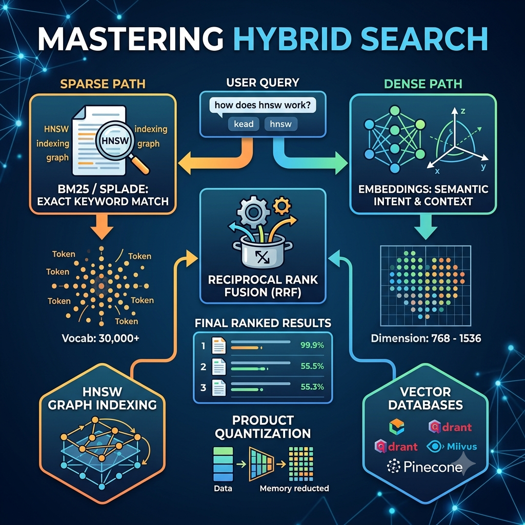
┌────────────────────────────────────────────────────────────────────────┐
│ HYBRID SEARCH ARCHITECTURE │
│ │
│ User Query │
│ │ │
│ ┌─────────────────────┴─────────────────────┐ │
│ ▼ ▼ │
│ ┌─────────────────┐ ┌─────────────────┐ │
│ │ Sparse Path │ │ Dense Path │ │
│ │ (BM25 / SPLADE)│ │ (Embeddings) │ │
│ │ Exact Keywords │ │ Semantic Intent │ │
│ └────────┬────────┘ └────────┬────────┘ │
│ │ │ │
│ └─────────────────────┬─────────────────────┘ │
│ ▼ │
│ ┌─────────────────────┐ │
│ │ Reciprocal Rank │ │
│ │ Fusion (RRF) │ │
│ └──────────┬──────────┘ │
│ ▼ │
│ Final Ranked Search Results │
└────────────────────────────────────────────────────────────────────────┘
Search technology has undergone a fundamental transformation. For decades, relational databases and search engines relied on exact lexical matching—matching query keywords against inverted indexes using algorithms like BM25 and TF-IDF. While fast and precise for exact alphanumeric searches, lexical search struggles with semantic understanding, synonyms, and multi-modal query intent.
The rise of high-dimensional vector representations changed the landscape. By embedding text, images, and audio into continuous vector spaces, vector databases allow applications to search by semantic meaning using nearest-neighbor search algorithms.
However, relying solely on vector embeddings creates new operational problems: pure dense search can miss exact SKU numbers, proper nouns, and specific technical terms.
To achieve production-grade accuracy at scale, modern data engineers build Hybrid Search Architectures that combine the precision of sparse keyword indexing with the contextual depth of dense vector embeddings.
💡 Key Takeaways
- Sparse vs. Dense: Sparse vectors (BM25) excel at exact keyword precision, while dense vectors (embeddings) capture semantic meaning and underlying context.
- HNSW Graph Indexing: Hierarchical Navigable Small World graphs enable sub-linear, approximate nearest neighbor (ANN) searches across millions of high-dimensional vectors.
- Hybrid Search Fusion: Reciprocal Rank Fusion (RRF) merges disparate relevance scores from sparse and dense retrieval streams into a unified, highly accurate rank list.
- Memory Optimization: Product Quantization (PQ) and Scalar Quantization (SQ) compress vector footprints, allowing massive datasets to fit cost-effectively in RAM.
Dense Embeddings vs. Sparse Tokens: Why Single-Vector Engines Fall Short
Understanding when to leverage sparse versus dense vector representations is essential for designing resilient data retrieval systems.
┌────────────────────────────────────────────────────────────────────────┐
│ SPARSE VS. DENSE VECTOR MATCHING │
│ │
│ SPARSE VECTORS (BM25 / SPLADE) DENSE VECTORS (EMBEDDINGS) │
│ ┌─────────────────────────────┐ ┌───────────────────────────┐ │
│ │ Dimension: 30,000+ (Vocab) │ │ Dimension: 768 – 1536 │ │
│ │ Values: Mostly Zeros (0.0) │ │ Values: Continuous Floats │ │
│ │ Strong at: Part Numbers, │ │ Strong at: Conceptual │ │
│ │ Proper Nouns, Exact IDs │ │ Context, Synonyms, Intent │ │
│ └─────────────────────────────┘ └───────────────────────────┘ │
└────────────────────────────────────────────────────────────────────────┘
The Limits of Pure Vector Search
Imagine a user searching an e-commerce catalog for the keyword “Part #A994-B”.
- A Dense Vector Model transforms this query string into a 1536-dimensional array of floating-point numbers. Because the model prioritizes conceptual meaning over exact characters, it might return general auto parts rather than the specific component with that exact serial number.
- A Sparse Lexical Engine maps the exact query string directly to its corresponding inverted index entry, instantly locating “Part #A994-B” with pinpoint accuracy.
Conversely, if a user queries “affordable battery-powered lawn mower”, a lexical search misses relevant products titled “Cordless Electric Grass Cutter” because there is no direct keyword overlap. The dense vector model handles this effortlessly because both phrases occupy similar locations in the semantic vector space.
Production systems require both capabilities operating in parallel.
Inside Vector Indexing: Demystifying HNSW and Quantization
Searching every vector in a database sequentially (exact $k$-Nearest Neighbors or $k$-NN) requires calculating the distance across millions of high-dimensional vectors for every query. This approach scales linearly $O(N \cdot d)$ and quickly becomes too slow for production environments.
To achieve sub-second query response times, vector engines rely on Approximate Nearest Neighbor (ANN) indexing. The industry standard index structure is HNSW (Hierarchical Navigable Small World) graphs.
HNSW MULTI-LAYER GRAPH STRUCTURE
Layer 2 (Express Route) o————————–> o
│ │
Layer 1 (Medium Hop) o———–> o ————>o
│ │ │
Layer 0 (Dense Graph) o—> o —> o —> o —> o
How HNSW Graph Routing Works
HNSW structures vector datasets into a multi-layer graph, drawing inspiration from the “skip list” data structure:
- Top Layers (Sparse Routing): The search begins at the top layer, which contains long-range link connections between distantly separated vector nodes. The engine traverses these express paths quickly to navigate to the general neighborhood of the target query vector.
- Lower Layers (Dense Local Search): Once the query gets close to the candidate vector neighborhood, execution drops down through progressively denser graph layers to pinpoint the closest vector neighbors.
- Time Complexity: HNSW reduces search complexity from $O(N)$ down to logarithmic time $O(\log N)$, enabling millisecond retrieval across billions of vectors.
Vector Compression: Scalar & Product Quantization
Storing raw 1536-dimensional vector arrays in Uncompressed 32-bit Floating Point format (fp32) consumes 6 KB of RAM per single vector. A dataset of 100 million vectors requires roughly 600 GB of pure memory just to host the raw vector representations.
Data engineers apply Quantization techniques to compress these vectors while maintaining high search accuracy:
- Scalar Quantization (SQ8): Converts 32-bit floats (fp32) down to 8-bit integers (int8), reducing memory consumption by 75% with negligible impact on retrieval recall.
- Product Quantization (PQ): Splits high-dimensional vectors into smaller sub-vectors and maps them to cluster centroids, achieving up to a 95% memory reduction to support massive scale on reduced hardware infrastructure.
Hands-On Implementation: Building a Hybrid Search Engine with Python
Let me show you how to implement a production-grade Hybrid Search pipeline in Python. We will combine lexical sparse search (BM25) with dense vector search (embeddings) and merge the outputs using Reciprocal Rank Fusion (RRF).
Complete Hybrid Search Implementation (hybrid_search.py)
Python
import numpy as np
from typing import List, Dict, Any
from rank_bm25 import BM25Okapi
from sentence_transformers import SentenceTransformer
class HybridSearchEngine:
“””Production-grade hybrid search pipeline merging sparse BM25 and dense vector search.”””
def __init__(self, model_name: str = “all-MiniLM-L6-v2”):
print(“[INIT] Loading Dense Embedding Model…”)
self.encoder = SentenceTransformer(model_name)
self.documents: List[Dict[str, Any]] = []
self.dense_embeddings: np.ndarray = np.array([])
self.bm25_engine: BM25Okapi = None
def index_documents(self, docs: List[Dict[str, Any]]):
“””Indexes raw document collections into sparse and dense structures.”””
self.documents = docs
corpus_texts = [doc[“text”] for doc in docs]
# 1. Build Sparse Index (BM25 Tokenization)
tokenized_corpus = [text.lower().split(” “) for text in corpus_texts]
self.bm25_engine = BM25Okapi(tokenized_corpus)
# 2. Build Dense Embedding Vectors
print(f”[INDEXING] Generating dense vectors for {len(docs)} documents…”)
embeddings = self.encoder.encode(corpus_texts, convert_to_numpy=True)
# Normalize vectors for fast Cosine Distance computation via Dot Product
norms = np.linalg.norm(embeddings, axis=1, keepdims=True)
self.dense_embeddings = embeddings / norms
print(“[INDEXING] Complete.”)
def search(self, query: str, top_k: int = 3, alpha: float = 60.0) -> List[Dict[str, Any]]:
“””Executes parallel sparse and dense searches, merging results via Reciprocal Rank Fusion.”””
# — PATH A: Sparse BM25 Retrieval —
tokenized_query = query.lower().split(” “)
bm25_scores = self.bm25_engine.get_scores(tokenized_query)
sparse_ranked_indices = np.argsort(bm25_scores)[::-1]
# — PATH B: Dense Vector Retrieval —
query_vector = self.encoder.encode([query], convert_to_numpy=True)
query_vector = query_vector / np.linalg.norm(query_vector)
# Calculate Cosine Similarities via Dot Product
dense_scores = np.dot(self.dense_embeddings, query_vector.T).flatten()
dense_ranked_indices = np.argsort(dense_scores)[::-1]
# — PATH C: Reciprocal Rank Fusion (RRF) —
rrf_scores: Dict[int, float] = {}
# Accumulate Sparse RRF Ranks
for rank, idx in enumerate(sparse_ranked_indices):
rrf_scores[idx] = rrf_scores.get(idx, 0.0) + (1.0 / (alpha + rank + 1))
# Accumulate Dense RRF Ranks
for rank, idx in enumerate(dense_ranked_indices):
rrf_scores[idx] = rrf_scores.get(idx, 0.0) + (1.0 / (alpha + rank + 1))
# Sort final fusion results
final_sorted_indices = sorted(rrf_scores.keys(), key=lambda i: rrf_scores[i], reverse=True)[:top_k]
results = []
for idx in final_sorted_indices:
results.append({
“id”: self.documents[idx][“id”],
“text”: self.documents[idx][“text”],
“rrf_score”: round(rrf_scores[idx], 5)
})
return results
if __name__ == “__main__”:
raw_docs = [
{“id”: “DOC-101”, “text”: “High speed battery powered electric lawn mower with steel blade.”},
{“id”: “DOC-102”, “text”: “Model X-400 battery charger for high capacity cordless tools.”},
{“id”: “DOC-103”, “text”: “Manual hand push grass cutter for small residential gardens.”}
]
engine = HybridSearchEngine()
engine.index_documents(raw_docs)
query_string = “electric grass cutting tool”
print(f”\n[QUERY]: ‘{query_string}'”)
search_results = engine.search(query=query_string, top_k=2)
for rank, res in enumerate(search_results, start=1):
print(f”Rank {rank} | ID: {res[‘id’]} | RRF Score: {res[‘rrf_score’]} | Content: {res[‘text’]}”)
Reciprocal Rank Fusion (RRF) Explained
RRF eliminates the challenge of combining incompatible metric scales (such as unbounded BM25 scores versus bounded cosine similarity floats) by converting raw scores into positional rank integers:
$$RRF\_Score(d \in D) = \sum_{m \in M} \frac{1}{k + r_m(d)}$$
Where $M$ represents the search systems (sparse and dense), $r_m(d)$ is document $d$’s rank position within model $m$, and $k$ is a smoothing constant (typically set to $60.0$).
Evaluating Production Vector Databases
Data engineering teams can select from several purpose-built vector databases depending on their infrastructure requirements:
| Vector Database | Architecture Model | Quantization Support | Best Infrastructure Use Case |
| Qdrant | Native Rust Core | SQ8, PQ, Binary Quantization | High-throughput, low-latency cloud systems |
| Milvus | Distributed Cloud-Native | Comprehensive (SQ/PQ/Scalar) | Enterprise-scale billions-vector workloads |
| Pinecone | Fully Managed Serverless | Managed Internally | Zero-Ops rapid development pipelines |
| pgvector | PostgreSQL Extension | HNSW / IVFFlat | Teams extending existing PostgreSQL setups |
Frequently Asked Questions (FAQ)
What is the difference between Cosine Distance, Dot Product, and Euclidean Distance ($L2$)?
- Euclidean Distance ($L2$): Measures the straight-line distance between two point coordinates in vector space. Sensitive to absolute vector magnitudes.
- Cosine Similarity: Measures the angle between two directional vectors, ignoring absolute scale or document length.
- Dot Product: Measures both vector angle and magnitude. When input vectors are unit-normalized to length $1.0$, Dot Product yields results mathematically identical to Cosine Similarity while executing faster on modern CPU architectures.
How does Filtering work inside a Vector Database?
Vector databases use Single-Pass Payload Filtering. Instead of filtering metadata after a vector search (which risks dropping relevant candidate results), engines like Qdrant and Milvus evaluate metadata filter conditions during graph traversal, ignoring non-matching nodes on the fly.
What is Binary Quantization (BQ)?
Binary Quantization is an aggressive vector compression technique that converts every 32-bit floating-point dimension into a single binary bit ($0$ or $1$) based on whether its value is positive or negative. This compresses vectors by 96.8% and uses ultra-fast CPU Hamming distance instructions for execution.
Conclusion & Action Steps
Relying on a single search retrieval paradigm is no longer sufficient for modern applications. By combining sparse lexical precision with dense semantic understanding in a unified Hybrid Search Engine, data engineers can build resilient, high-recall search systems that handle complex queries accurately.
Next Steps for Data Engineers:
- Benchmark your current search setup against a representative query evaluation set containing exact SKUs, technical jargon, and natural language concepts.
- Integrate an open-source vector engine like Qdrant or pgvector alongside your existing text database.
- Implement Reciprocal Rank Fusion (RRF) to combine sparse and dense search pipelines into a single ranked stream.