Quantum Computing for Software Engineers: Qubits, Algorithms, and Cloud Frameworks
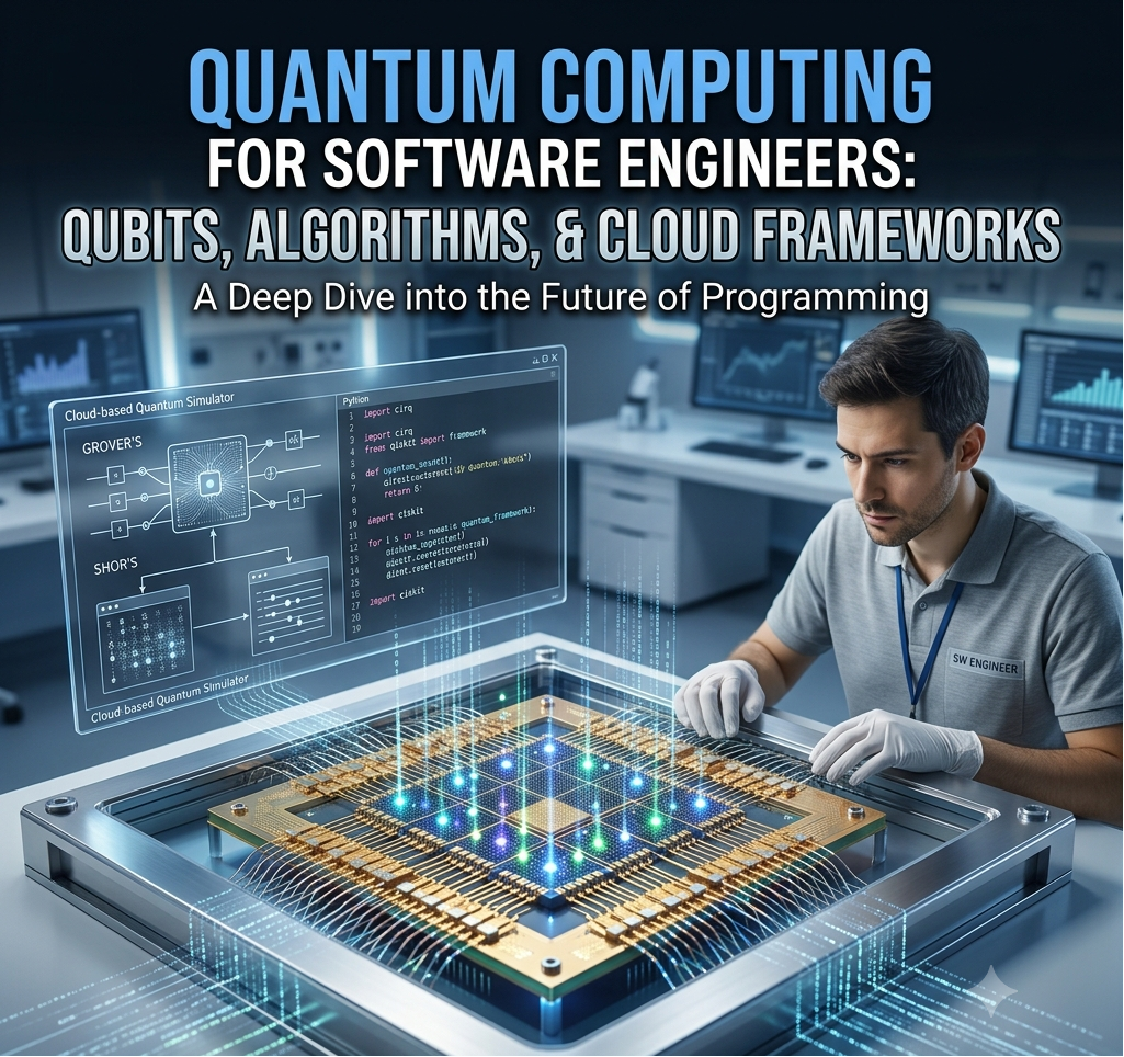
Meta Description: Understand Quantum Computing from a software engineering perspective. Learn Qubit physics, superposition, entanglement, and Qiskit programming.
┌────────────────────────────────────────────────────────────────────────┐
│ CLASSICAL BITS VS. QUANTUM QUBITS │
│ │
│ CLASSICAL BIT (Deterministic) │
│ ┌───────────────────────────┐ • Value is strictly 0 OR 1 │
│ │ 0 OR 1 │ • Switches deterministically │
│ └───────────────────────────┘ │
│ │
│ QUANTUM QUBIT (Bloch Sphere) │
│ |0⟩ (North) │
│ │ • $|\psi\rangle = \alpha|0\rangle + \beta|1\rangle$ │
│ .–┼–. • Holds continuous superposition │
│ / │ \ • Entangles with other qubits │
│ | o—-+—> Y • Collapses upon measurement │
│ \ / / │
│ ‘–┼–‘ │
│ |1⟩ (South) │
└────────────────────────────────────────────────────────────────────────┘
For decades, modern software architecture has relied on classical computing principles. Classical transistors store state deterministically as either a binary 0 or 1. Every software abstraction—from low-level assembly to distributed microservices—ultimately executes on these boolean operations.
However, classical processors struggle with specific classes of complex mathematical problems. Calculating molecular folding configurations, optimizing global supply chain logistics, and factoring massive prime integers scale exponentially on classical architectures ($O(2^n)$), requiring supercomputers to run for millennia to compute solutions.
Quantum Computing shifts the computational paradigm. By harnessing principles of quantum mechanics—specifically superposition, quantum entanglement, and quantum interference—quantum algorithms solve previously intractable problems in polynomial time.
For software engineers, quantum computing is transitioning from physics research into an accessible programming model powered by open-source SDKs and cloud-hosted quantum hardware.
💡 Key Takeaways
- Superposition & Entanglement: Qubits exist in linear combinations of $\vert{}0\rangle$ and $\vert{}1\rangle$ simultaneously, while entanglement links qubit states instantaneously regardless of physical distance.
- Quantum Gates as Matrices: Quantum programs are represented as unitary matrix operations applied to complex state vectors.
- Exponential State Representation: $N$ entangled qubits represent $2^N$ complex probability amplitudes simultaneously in memory.
- Cloud Quantum Frameworks: Frameworks like IBM’s Qiskit allow software developers to write quantum circuits in Python and execute them on physical Quantum Processing Units (QPUs).
Quantum Mechanics Primitives: Superposition & Entanglement
To program quantum processors, developers must understand three fundamental quantum mechanical principles:
┌────────────────────────────────────────────────────────────────────────┐
│ THE THREE QUANTUM PRIMITIVES │
│ │
│ 1. Superposition : A qubit holds a probability continuum between │
│ |0⟩ and |1⟩ until measured. │
│ 2. Entanglement : Two qubits become interconnected; measuring one │
│ instantly determines the state of the other. │
│ 3. Interference : Quantum gates amplify correct answers while │
│ canceling out incorrect computational paths. │
└────────────────────────────────────────────────────────────────────────┘
1. Superposition
A classical bit exists in a state of $0$ or $1$. A qubit (quantum bit) is represented mathematically as a normalized vector in a two-dimensional complex Hilbert space:
$$\vert{}\psi\rangle = \alpha\vert{}0\rangle + \beta\vert{}1\rangle$$
Where $\alpha$ and $\beta$ are complex numbers representing probability amplitudes. The sum of their squared probabilities must equal 1:
$$\vert{}\alpha\vert{}^2 + \vert{}\beta\vert{}^2 = 1$$
While unobserved, a qubit holds a continuum of potential states. However, the moment an application measures the qubit, its superposition state collapses deterministically into either a classical 0 (with probability $\vert{}\alpha\vert{}^2$) or 1 (with probability $\vert{}\beta\vert{}^2$).
2. Quantum Entanglement
When two qubits interact, they can become entangled. The state of an entangled system cannot be decomposed into separate single-qubit descriptions.
For example, consider the entangled Bell State $\vert{}\Phi^+\rangle$:
$$\vert{}\Phi^+\rangle = \frac{\vert{}00\rangle + \vert{}11\rangle}{\sqrt{2}}$$
In this state, neither individual qubit has a definite value. However, if Qubit A is measured and observed as $\vert{}0\rangle$, Qubit B instantly collapses to $\vert{}0\rangle$ as well, regardless of the physical distance separating them. This property enables parallel computational pathways across quantum registers.
The Exponential Scale Advantage
The computational capability of a quantum processor grows exponentially relative to its qubit count:
┌────────────────────────────────────────────────────────────────────────┐
│ EXPONENTIAL QUANTUM STATE CAPACITY │
│ │
│ • 1 Qubit = 2 Amplitudes (2¹) │
│ • 10 Qubits = 1,024 Amplitudes (2¹⁰) │
│ • 50 Qubits = ~1.12 × 10¹⁵ Amplitudes (Exceeds high-end RAM) │
│ • 300 Qubits = 2³⁰⁰ Amplitudes (Exceeds atoms in visible universe) │
└────────────────────────────────────────────────────────────────────────┘
While $N$ classical bits hold exactly $N$ values at a time, $N$ entangled qubits store $2^N$ complex probability amplitudes simultaneously. A quantum algorithm processes all $2^N$ states in parallel using single gate operations.
Hands-On Implementation: Building a Quantum Circuit with Qiskit & Python
Let’s write a complete quantum program using IBM’s Qiskit framework. We will construct a 2-qubit quantum circuit, place Qubit 0 into superposition using a Hadamard Gate, entangle it with Qubit 1 using a Controlled-NOT (CNOT) Gate, and measure the output state.
Python
# Dependencies: pip install qiskit qiskit-aer
import numpy as np
from qiskit import QuantumCircuit
from qiskit_aer import AerSimulator
def execute_quantum_entanglement_circuit():
“””
Constructs and executes a 2-qubit Bell State Entanglement Circuit.
“””
print(“[INIT] Constructing 2-Qubit Quantum Circuit…”)
# Initialize circuit with 2 Qubits and 2 Classical Readout Bits
qc = QuantumCircuit(2, 2)
# Step 1: Apply Hadamard (H) Gate to Qubit 0
# Moves Qubit 0 from state |0> into equal superposition: (|0> + |1>) / sqrt(2)
qc.h(0)
# Step 2: Apply Controlled-NOT (CNOT) Gate with Control=Qubit 0, Target=Qubit 1
# Entangles Qubit 1 directly with Qubit 0
qc.cx(0, 1)
# Step 3: Measure Qubits 0 and 1 into Classical Bits 0 and 1
qc.measure([0, 1], [0, 1])
# Display ASCII representation of the Quantum Circuit
print(“\n— QUANTUM CIRCUIT DIAGRAM —“)
print(qc.draw(output=’text’))
# Step 4: Execute Circuit on Local Quantum Aer Simulator
print(“\n[EXECUTION] Simulating circuit across 1,000 shots…”)
simulator = AerSimulator()
job = simulator.run(qc, shots=1000)
result = job.result()
counts = result.get_counts(qc)
print(“\n— QUANTUM MEASUREMENT RESULTS —“)
for state, frequency in counts.items():
percentage = (frequency / 1000) * 100
print(f”State |{state}⟩ : {frequency} occurrences ({percentage:.1f}%)”)
if __name__ == “__main__”:
execute_quantum_entanglement_circuit()
Circuit Execution Breakdown
┌───┐ ┌─┐
q_0: ──┤ H ├──■──┤M├───
└───┘┌─┴─┐└┬┘┌─┐
q_1: ───────┤ X ├─┼─┤M├
└───┘ └┴┘└┬┘
c: ═══════════════════╧═
- qc.h(0) (Hadamard Gate): Transforms Qubit 0 into a $50/50$ superposition state.
- qc.cx(0, 1) (CNOT Gate): Flips Qubit 1 if and only if Qubit 0 evaluates to $\vert{}1\rangle$.
- Results: The output counts show exclusively states 00 (~50%) and 11 (~50%). Intermediate states 01 and 10 never occur, proving the qubits are entangled.
Key Quantum Algorithms & Industrial Applications
Quantum computing provides speedups for targeted mathematical domains:
┌────────────────────────────────────────────────────────────────────────┐
│ DOMAINS OF QUANTUM ACCELERATION │
│ │
│ • Cryptography & Security : Shor’s Algorithm (Polynomial Factoring)│
│ • Database & Unstructured : Grover’s Algorithm (Quadratic Speedup) │
│ • Chemistry & Materials : VQE (Variational Quantum Eigensolver) │
│ • Financial Optimization : QAOA (Optimization Algorithms) │
└────────────────────────────────────────────────────────────────────────┘
| Quantum Algorithm | Classical Complexity | Quantum Complexity | Target Application |
| Shor’s Algorithm | Exponential $O(e^{\sqrt{\log N}})$ | Polynomial $O((\log N)^3)$ | Breaking RSA public-key encryption |
| Grover’s Search | Linear $O(N)$ | Quadratic $O(\sqrt{N})$ | Unstructured database search |
| VQE (Variational Quantum Eigensolver) | Exponential $O(2^N)$ | Hybrid Quantum-Classical $O(N^k)$ | Molecular structure & battery design |
| QAOA (Quantum Approximate Optimization) | NP-Hard / Exponential | Hybrid Accelerated | Logistics & Portfolio Optimization |
The NISQ Era and Post-Quantum Cryptography (PQC)
We currently live in the NISQ (Noisy Intermediate-Scale Quantum) era. Modern quantum processors contain dozens to hundreds of physical qubits, but they remain prone to quantum decoherence and environmental noise.
┌────────────────────────────────────────────────────────────────────────┐
│ THE POST-QUANTUM THREAT TIMELINE │
│ │
│ Today : “Harvest Now, Decrypt Later” Attacks │
│ Adversaries capture encrypted public data streams. │
│ │
│ Future: Cryptographically Relevant Quantum Computer (CRQC) Arrives │
│ Shor’s Algorithm factors RSA/ECC keys, decrypting historical │
│ data retroactively. │
└────────────────────────────────────────────────────────────────────────┘
Engineering Imperative: Post-Quantum Cryptography (PQC)
Because Shor’s Algorithm breaks asymmetric cryptography (RSA, ECC, Diffie-Hellman), standards bodies like NIST have finalized Post-Quantum Cryptography (PQC) standards (e.g., ML-KEM and ML-DSA). Software engineering teams must prepare by transitioning application security layers to quantum-resistant lattice algorithms.
Frequently Asked Questions (FAQ)
Will Quantum Computers replace classical CPUs and GPUs?
No. Quantum computers act as specialized accelerators (similar to GPUs) for specific mathematical workloads. Standard tasks like web hosting, UI rendering, database CRUD operations, and logic processing run more efficiently on classical architectures.
What is Quantum Decoherence?
Decoherence occurs when a qubit loses its quantum state due to thermal fluctuations, electromagnetic radiation, or environmental noise. When decoherence happens, superposition collapses prematurely, introducing errors into quantum calculations.
How can developers test quantum programs without quantum hardware?
Frameworks like Qiskit, Cirq, and Pennylane include high-performance local classical simulators (AerSimulator). Developers can run and debug circuits containing up to ~25-30 qubits locally on standard developer workstations before submitting jobs to cloud QPUs via services like IBM Quantum, AWS Braket, or Azure Quantum.
Conclusion & Action Steps
Quantum computing introduces a paradigm shift in computational complexity. As hardware matures beyond the NISQ era, software engineers who understand qubit mechanics, quantum gate operations, and hybrid programming models will be uniquely positioned to build the next generation of accelerated applications.
Next Steps for Software Engineers:
- Install Python quantum development tools (pip install qiskit qiskit-aer).
- Run a local Bell-State circuit simulator to visualize qubit superposition and entanglement.
- Review your organization’s security posture and plan the migration of sensitive RSA/ECC encryption keys to Post-Quantum Cryptography (PQC) algorithms.