Graph Neural Networks (GNNs): Unlocking Structured Data in Machine Learning
Meta Description: Explore Graph Neural Networks (GNNs). Learn how Message Passing, Spatial/Spectral Convolutions, and PyTorch Geometric unlock non-Euclidean data.
┌────────────────────────────────────────────────────────────────────────┐
│ EUCLIDEAN VS. NON-EUCLIDEAN DATA STRUCTURES │
│ │
│ EUCLIDEAN DATA (Grid / Sequence) │
│ ┌───┬───┬───┐ • Images (2D Pixel Grid) │
│ ├───┼───┼───┤ • Text (1D Word Sequences) │
│ └───┴───┴───┘ • Fixed N-dimensional structure │
│ │
│ NON-EUCLIDEAN DATA (Graphs / Networks) │
│ (A) ─────── (B) │
│ ╱ ╲ ╱ • Social Networks & Fraud Rings │
│ (C)───(D)───(E) • Molecular Structures & Drug Discovery │
│ • Knowledge Graphs & Financial Chains │
└────────────────────────────────────────────────────────────────────────┘
Traditional deep learning models excel at processing data structured in Euclidean space. Convolutional Neural Networks (CNNs) process 2D pixel grids in images, and Recurrent Neural Networks (RNNs) or Transformers process 1D sequential tokens in natural language.
However, many real-world datasets do not fit neatly into flat grids or linear sequences. Molecular structures, financial transaction networks, social interaction graphs, telecommunication topologies, and recommendation engines exist in Non-Euclidean space. In these domains, data points are defined by variable connectivity, irregular topology, and complex relational dependencies.
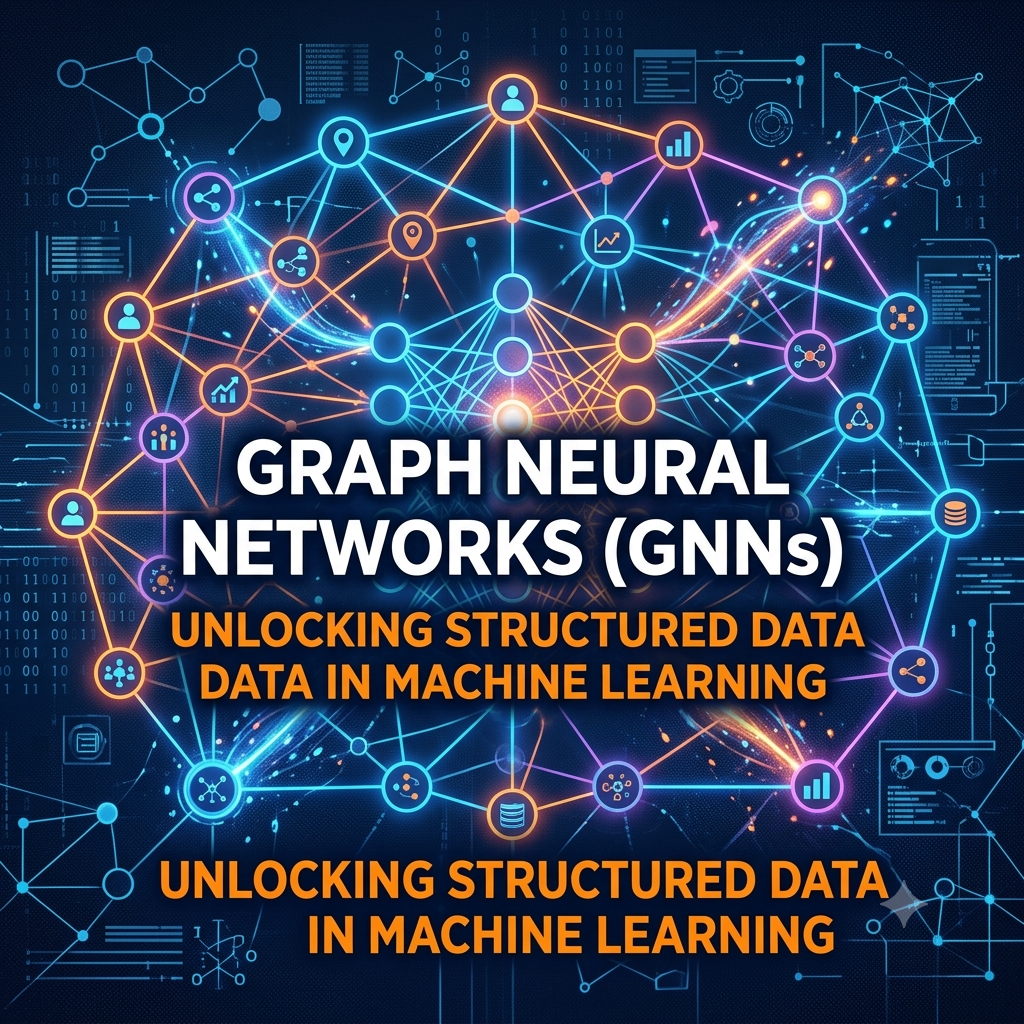
Graph Neural Networks (GNNs) bridge this gap. By extending deep learning primitives to graph-structured data, GNNs enable machine learning models to reason directly over nodes, edges, and global graph contexts—unlocking breakthrough capabilities in drug discovery, fraud detection, and system optimization.
💡 Key Takeaways
- Non-Euclidean Representation: GNNs capture relational structures and node connections that standard matrix-based deep learning models ignore.
- Message Passing Paradigm: The core operation of GNNs involves iteratively aggregating features from neighboring nodes to update target node representations.
- Permutation Invariance: Graph operators produce identical output embeddings regardless of how nodes and edges are ordered or indexed in memory.
- Node, Edge & Graph-Level Tasks: GNNs scale across diverse tasks, from predicting individual node categories (e.g., fraud accounts) to scoring whole-graph properties (e.g., drug toxicity).
Why Standard Deep Learning Models Fail on Graphs
To understand why GNNs are necessary, consider attempting to pass a social network graph into a traditional Multi-Layer Perceptron (MLP) or CNN:
┌────────────────────────────────────────────────────────────────────────┐
│ GRAPH REPRESENTATION CHALLENGES │
│ │
│ 1. Variable Neighborhood Sizes : Node A has 2 edges, Node B has 500 │
│ 2. Lack of Fixed Spatial Order : No top/bottom/left/right in graphs │
│ 3. Permutation Sensitivity : Changing matrix order alters output │
└────────────────────────────────────────────────────────────────────────┘
- Permutation Sensitivity: Standard neural network layers treat input vectors as ordered sequences. If you reorder the rows of a graph’s adjacency matrix, a standard MLP interprets it as an entirely new dataset, even though the underlying graph topology remains identical.
- Dynamic Topology: Images have fixed pixel dimensions, but graphs have variable numbers of neighbors per node. A node might connect to a single neighbor or to millions of hubs simultaneously.
- Loss of Relational Context: Flattening a graph adjacency matrix into a flat feature vector destroys local topological information and leads to high-dimensional, sparse representations that struggle to generalize.
The Core Primitive: The Message Passing Framework
Modern Graph Neural Networks operate using the Message Passing paradigm (also known as Spatial Graph Convolutions).
During each message passing layer, every node collects feature vectors from its immediate structural neighbors, combines them using a permutation-invariant aggregation operator, and updates its internal hidden state representation.
┌────────────────────────────────────────────────────────────────────────┐
│ MESSAGE PASSING PHASE IN A GNN │
│ │
│ Neighbor Nodes Aggregation Target Node │
│ ┌──────────────┐ ┌────────────────┐ ┌─────────────┐ │
│ │ Node B State │───Message──>│ │ │ │ │
│ └──────────────┘ │ │ │ │ │
│ ┌──────────────┐ │ Sum / Mean / ├────>│ Node A │ │
│ │ Node C State │───Message──>│ Max Aggregator │ │ Updated │ │
│ └──────────────┘ │ │ │ State │ │
│ ┌──────────────┐ │ │ │ │ │
│ │ Node D State │───Message──>│ │ │ │ │
│ └──────────────┘ └────────────────┘ └─────────────┘ │
└────────────────────────────────────────────────────────────────────────┘
The 3 Mathematical Steps of Message Passing
For a graph $G = (V, E)$, the hidden representation $h_v^{(l)}$ of node $v$ at layer $l$ updates via three sequential operations:
- Message Generation: Compute a message vector $m_{u \to v}^{(l)}$ from each neighboring node $u \in \mathcal{N}(v)$:
$$m_{u \to v}^{(l)} = \text{MSG}^{(l)}\left(h_u^{(l-1)}, h_v^{(l-1)}, e_{uv}\right)$$
- Aggregation: Aggregate messages from all incoming neighbors using a permutation-invariant function (such as $\sum$, $\text{Mean}$, or $\text{Max}$):
$$M_v^{(l)} = \text{AGG}^{(l)}\left( \left\{ m_{u \to v}^{(l)} : u \in \mathcal{N}(v) \right\} \right)$$
- State Update: Combine the aggregated neighborhood representation $M_v^{(l)}$ with the node’s previous state $h_v^{(l-1)}$ to produce the updated embedding:
$$h_v^{(l)} = \text{UPDATE}^{(l)}\left(h_v^{(l-1)}, M_v^{(l)}\right)$$
With $k$ stacked message passing layers, each node gathers contextual information from all neighbors located up to $k$-hops away in the graph topology.
Hands-On Implementation: Node Classification with PyTorch Geometric
Let’s implement a Graph Convolutional Network (GCN) using torch_geometric to perform node classification (e.g., detecting fraudulent accounts within an interaction network).
Python
import torch
import torch.nn as nn
import torch.nn.functional as F
from torch_geometric.nn import GCNConv
from torch_geometric.data import Data
class GraphFraudClassifier(nn.Module):
“””
Two-layer Graph Convolutional Network (GCN) for Node Classification.
“””
def __init__(self, in_features: int, hidden_dim: int, num_classes: int):
super(GraphFraudClassifier, self).__init__()
# First Graph Convolution Layer (Gathers 1-hop neighborhood)
self.conv1 = GCNConv(in_features, hidden_dim)
# Second Graph Convolution Layer (Gathers 2-hop neighborhood)
self.conv2 = GCNConv(hidden_dim, num_classes)
def forward(self, x: torch.Tensor, edge_index: torch.Tensor) -> torch.Tensor:
“””
Args:
x: Node feature matrix of shape [Num_Nodes, In_Features]
edge_index: Graph connectivity matrix of shape [2, Num_Edges]
“””
# Layer 1: Spatial Graph Convolution + Non-Linearity + Dropout
x = self.conv1(x, edge_index)
x = F.relu(x)
x = F.dropout(x, p=0.2, training=self.training)
# Layer 2: Final Layer mapping to Class Logits
x = self.conv2(x, edge_index)
return F.log_softmax(x, dim=1)
# — SYNTHETIC GRAPH DATA SETUP —
# 4 Nodes (Accounts), 3 Edge Connections (Transactions)
node_features = torch.tensor([
[-0.5, 0.2, 1.1], # Node 0
[ 1.2, -0.8, 0.4], # Node 1
[ 0.1, 0.9, -0.3], # Node 2
[-1.1, -0.4, 0.8] # Node 3
], dtype=torch.float)
# Directed Edges: 0->1, 1->2, 2->3, 3->0
edge_connections = torch.tensor([
[0, 1, 2, 3],
[1, 2, 3, 0]
], dtype=torch.long)
# Binary Labels: 0 = Legitimate Account, 1 = Fraudulent Account
labels = torch.tensor([0, 1, 0, 1], dtype=torch.long)
# PyTorch Geometric Data Container
graph_dataset = Data(x=node_features, edge_index=edge_connections, y=labels)
# — MODEL INITIALIZATION & FORWARD PASS —
model = GraphFraudClassifier(in_features=3, hidden_dim=16, num_classes=2)
model.eval()
with torch.no_grad():
predictions = model(graph_dataset.x, graph_dataset.edge_index)
predicted_classes = predictions.argmax(dim=1)
print(“[GNN INFERENCE COMPLETE]”)
for node_id, cls in enumerate(predicted_classes):
print(f”Node {node_id} -> Predicted Category: {cls.item()}”)
Comparing GNN Architectures: GCN vs. GAT vs. GraphSAGE
Over time, several key GNN variants have emerged to address specific graph learning challenges:
┌────────────────────────────────────────────────────────────────────────┐
│ GNN ARCHITECTURE EVOLUTION │
│ │
│ GCN (Kipf & Welling) ──> GraphSAGE ──> GAT │
│ Fixed normalized Inductive neighborhood Dynamic │
│ neighborhood weights sampling for massive graphs Attention │
└────────────────────────────────────────────────────────────────────────┘
| Model Architecture | Key Innovation | Primary Use Case | Scaling Limitation |
| GCN (Graph Convolutional Net) | Symmetrically normalized adjacency matrix smoothing | Transductive node classification | Full-batch training requires full graph in RAM |
| GraphSAGE | Uniform neighborhood sampling & inductive generalization | Industrial graphs (Pinterest, Uber Eats) | Hyperparameter tuning needed for sample sizes |
| GAT (Graph Attention Net) | Dynamic attention weights assigned to neighboring edges | Chemical graphs & protein interaction | Higher computational and memory overhead |
Real-World Engineering Applications of GNNs
Graph Neural Networks have transitioned from academic research into foundational infrastructure across major technology domains:
┌────────────────────────────────────────────────────────────────────────┐
│ GNN INDUSTRIAL APPLICATIONS │
│ │
│ 1. Drug Discovery & Molecular Engineering (AlphaFold, MoleculeNet) │
│ 2. Financial Fraud Detection (Anti-Money Laundering Rings) │
│ 3. E-Commerce Recommendation Engines (User-Item Bipartite Graphs) │
│ 4. Traffic & Logistics Optimization (Google Maps Transit Prediction) │
└────────────────────────────────────────────────────────────────────────┘
- Anti-Money Laundering (AML): Financial institutions model accounts as nodes and money transfers as directed edges. GNNs detect complex “ring-shaped” laundering topologies that evade standard rule engines.
- Molecular Property Prediction: Atoms act as nodes, and covalent bonds act as edges. GNNs predict molecular binding affinity, toxicity, and chemical properties to accelerate drug discovery.
- Entity Recommendation Systems: E-commerce applications structure interactions as bipartite graphs connecting users to products. Models like Pinterest’s PinSage process billions of nodes to deliver personalized recommendations.
Frequently Asked Questions (FAQ)
What is the difference between Transductive and Inductive learning in GNNs?
- Transductive Learning: The model requires the entire graph structure (including test nodes without labels) during training. Standard GCNs are transductive.
- Inductive Learning: The model learns aggregation functions that generalize to completely unseen nodes or novel subgraphs that were not present during training. GraphSAGE is designed for inductive learning.
What is the “Oversmoothing” problem in Graph Neural Networks?
Oversmoothing occurs when stacking too many message-passing layers (typically more than 3 to 5 layers). As information propagates repeatedly across the graph, all node representations converge toward identical average vectors, drastically reducing classification performance. Techniques like residual connections, jumping knowledge networks, and pair-norm layers help mitigate oversmoothing.
How do GNNs scale to enterprise graphs containing billions of edges?
Large enterprise graphs cannot fit into single-GPU memory. Scale is achieved via Neighborhood Sampling (e.g., GraphSAGE), Graph Partitioning (e.g., Cluster-GCN), or distributed graph database engines (such as PyTorch Geometric Engine or DGL) that split graph topologies across distributed cluster nodes.
Conclusion & Action Steps
Graph Neural Networks provide a powerful framework for learning over complex, relational data structures. By capturing topological context and node features simultaneously through message passing, GNNs enable machine learning solutions across non-Euclidean domains.
Next Steps for ML Engineers:
- Install torch_geometric or dgl (Deep Graph Library) inside your Python environment.
- Formulate an existing domain problem as a graph (e.g., mapping user interactions, system dependencies, or transaction chains).
- Benchmark a standard baseline (like an XGBoost model operating on tabular features) against a 2-layer GraphSAGE or GCN pipeline to evaluate topological gains.