Advanced Database Internals: LSM-Trees, B-Trees, and Storage Engine Tradeoffs
Meta Description: Master advanced database internals. Compare B-Trees and LSM-Trees, explore write amplification, SSTables, WAL, and storage engine tradeoffs.
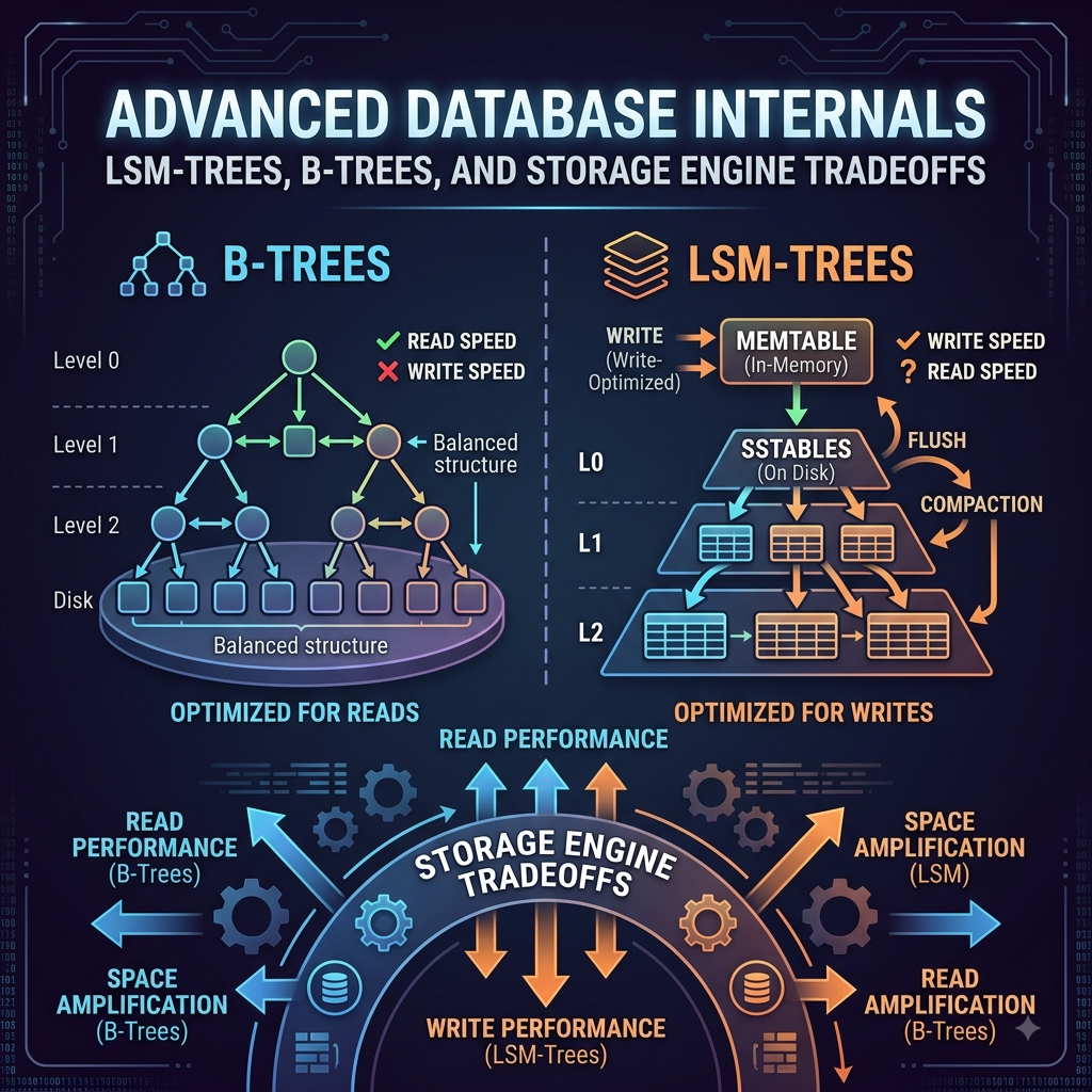
┌────────────────────────────────────────────────────────────────────────┐
│ B-TREE VS. LSM-TREE STORAGE │
│ │
│ B-TREE (In-Place Updates – Read-Optimized) │
│ ┌────────────────────────────────────────────────────────────────┐ │
│ │ Dynamic Page Tree (e.g., 8KB Pages) │ │
│ │ [ Root Node ] ──> [ Internal Node ] ──> [ Leaf Page (Overwritten) ]│ │
│ └────────────────────────────────────────────────────────────────┘ │
│ │
│ LSM-TREE (Append-Only Sequential Writes – Write-Optimized) │
│ ┌────────────────────────────────────────────────────────────────┐ │
│ │ RAM: [ MemTable (SkipList) ] ──> [ Write-Ahead Log (WAL) ] │
│ │ DISK: [ SSTable L0 ] ──> [ SSTable L1 ] ──> [ Compaction ] │ │
│ └────────────────────────────────────────────────────────────────┘ │
└────────────────────────────────────────────────────────────────────────┘
At the core of every relational or NoSQL database sits a crucial component: the Storage Engine. The storage engine manages how data structures are mapped between memory (RAM) and non-volatile storage media (SSDs/NVMe disks).
When designing high-throughput data systems, engineers often evaluate databases based on query languages or feature sets. However, long-term system performance—including read latency, write throughput, storage footprint, and hardware lifespan—is determined by the storage engine’s underlying data structure.
The modern storage engine landscape is divided into two primary design models: B-Trees (and their $B^+$-Tree variants), which favor in-place updates optimized for fast reads, and Log-Structured Merge-Trees (LSM-Trees), which leverage append-only sequential writes optimized for massive write ingest.
💡 Key Takeaways
- In-Place vs. Append-Only: B-Trees update fixed-size disk pages in place, while LSM-Trees buffer mutations in memory and write immutable sorted files sequentially.
- Hardware I/O Dynamics: LSM-Trees maximize SSD throughput by converting random write workloads into efficient sequential disk writes.
- The RUM Conjecture: Storage engine designs trade off Read Overhead, Update Overhead, and Memory Overhead—you cannot optimize all three simultaneously.
- Compaction Mitigates Space Amplification: LSM-Trees rely on background merging (compaction) to remove duplicate, stale, or deleted records from disk.
B-Trees: The Benchmark for Read-Heavy Workloads
Invented in 1970, the B-Tree (and the predominant $B^+$-Tree) remains the standard storage architecture for general-purpose relational database systems like MySQL (InnoDB), PostgreSQL, and SQLite.
┌────────────────────────────────────────────────────────────────────────┐
│ B+ TREE NODE LAYOUT │
│ │
│ [ Root Node: Keys 50, 100 ] │
│ ╱ │ ╲ │
│ ╱ │ ╲ │
│ [ Key < 50 ] ────┘ │ └─── [ Key >= 100 ] │
│ ▼ │
│ [ Key 50 <= K < 100 ] │
│ [ Leaf Page: 8KB ] │
│ ┌──────────────────┐ │
│ │ K:52 | V: “Alice”│ │
│ │ K:78 | V: “Bob” ├─ Pointer ─> [ Next Leaf ] │
│ └──────────────────┘ │
└────────────────────────────────────────────────────────────────────────┘
B-Tree Design Principles
- Fixed-Size Pages: B-Trees divide databases into fixed-size blocks (typically 4KB to 16KB pages). These pages map directly to hardware disk blocks.
- Balanced Tree Structure: A $B^+$-Tree guarantees that all leaf pages sit at equal depth, delivering deterministic logarithmic lookup complexity $O(\log N)$.
- In-Place Updates: When a record is updated or inserted, the storage engine locates the target 8KB leaf page on disk and overwrites its contents in place.
The Problem: Random I/O and Write Amplification
In-place updates introduce significant performance costs for write-heavy workloads:
- Random Disk I/O: Modifying small records scattered across different pages forces random I/O operations, which causes latency spikes on storage drives.
- Write Amplification Factor (WAF): Updating a single 10-byte field requires rewriting the entire 8KB page back to disk. This causes a high Write Amplification Factor ($\text{WAF} = \frac{\text{Bytes Written to Disk}}{\text{Bytes Requested by Application}}$), which degrades write performance and shortens SSD lifespans over time.
Log-Structured Merge-Trees (LSM-Trees): Built for Write Scale
To handle high-throughput write workloads, storage engines like RocksDB, LevelDB, Apache Cassandra, and ScyllaDB use Log-Structured Merge-Trees (LSM-Trees).
┌────────────────────────────────────────────────────────────────────────┐
│ LSM-TREE WRITE PATHWAY │
│ │
│ Write Request │
│ │ │
│ ├───( Sequential Append )───> [ Write-Ahead Log (WAL) ] │
│ │ │
│ └───( Sorted In-Memory )────> [ MemTable (SkipList) ] │
│ │ │
│ ( Flushes when full ) │
│ ▼ │
│ Disk Storage [ SSTable Level 0 ] │
│ [ Sorted Immutable File ] │
│ │ │
│ ( Background Compaction ) │
│ ▼ │
│ [ SSTable Level 1 ] │
└────────────────────────────────────────────────────────────────────────┘
LSM-Tree Write Workflow
- Write-Ahead Log (WAL): When a write arrives, it is appended to an on-disk Write-Ahead Log (WAL) sequentially. This guarantees durability in the event of power loss or process crashes.
- MemTable: Simultaneously, the record is inserted into an in-memory sorted structure called the MemTable (typically implemented as a SkipList or Red-Black Tree). This memory write runs with $O(\log N)$ latency.
- SSTable Flushing: When the MemTable fills up (e.g., reaches 64MB), it converts into an immutable structure and flushes sequentially to disk as a Sorted String Table (SSTable).
- SSTable Compaction: Because SSTables are immutable, updating a key simply writes a new entry to a new SSTable (or writes a “tombstone” marker for deletions). Background compaction processes merge overlapping SSTables to prune duplicate versions and re-establish sorted key ranges.
Hands-On Implementation: Building an In-Memory MemTable and SSTable Flush Engine in Python
Let’s implement a core component of an LSM-Tree storage engine: a sorted MemTable that flushes to disk as an immutable SSTable file with a sparse memory index.
Python
import os
import json
from typing import Dict, Optional, List
class SSTable:
“””Represents an immutable Sorted String Table (SSTable) file on disk.”””
def __init__(self, filepath: str, sparse_index: Dict[str, int]):
self.filepath = filepath
self.sparse_index = sparse_index # Maps sample keys to byte offsets for fast seek
def get(self, key: str) -> Optional[str]:
“””Performs index-assisted sparse search to locate a key on disk.”””
if not os.path.exists(self.filepath):
return None
# Determine binary file offset range using sparse index
keys = list(self.sparse_index.keys())
target_offset = 0
for k in keys:
if k <= key:
target_offset = self.sparse_index[k]
else:
break
# Seek directly into disk file to minimize I/O overhead
with open(self.filepath, ‘r’) as f:
f.seek(target_offset)
for line in f:
if not line.strip():
continue
record = json.loads(line)
if record[‘key’] == key:
return record[‘val’]
if record[‘key’] > key:
break # Sorted order guarantees key does not exist past this point
return None
class LSMMemTable:
“””In-memory buffer (MemTable) that flushes sorted key-value pairs to disk as SSTables.”””
def __init__(self, capacity_threshold: int = 3):
self.capacity_threshold = capacity_threshold
self.buffer: Dict[str, str] = {}
self.sstables: List[SSTable] = []
self.flush_count = 0
def put(self, key: str, val: str):
“””Inserts a key-value pair into the sorted MemTable, flushing if capacity is reached.”””
self.buffer[key] = val
print(f”[MEMTABLE INSERT] Key: ‘{key}’ -> Val: ‘{val}'”)
if len(self.buffer) >= self.capacity_threshold:
self._flush_to_sstable()
def _flush_to_sstable(self):
“””Flushes in-memory contents to disk in sorted order as an immutable SSTable.”””
self.flush_count += 1
filepath = f”sstable_level0_{self.flush_count}.db”
print(f”\n[FLUSHING MEMTABLE] Capacity reached. Writing immutable ‘{filepath}’ to disk…”)
# Sort keys to maintain strict SSTable ordering invariants
sorted_keys = sorted(self.buffer.keys())
sparse_index: Dict[str, int] = {}
with open(filepath, ‘w’) as f:
for idx, key in enumerate(sorted_keys):
byte_offset = f.tell()
# Create sparse index entry every 2 keys
if idx % 2 == 0:
sparse_index[key] = byte_offset
payload = json.dumps({“key”: key, “val”: self.buffer[key]})
f.write(payload + “\n”)
self.sstables.insert(0, SSTable(filepath, sparse_index))
self.buffer.clear()
print(f”[FLUSH COMPLETE] Created sparse index: {sparse_index}\n”)
def get(self, key: str) -> Optional[str]:
“””Reads key across storage layers (MemTable -> Recent SSTables -> Older SSTables).”””
# 1. Search in-memory MemTable first (Zero Latency)
if key in self.buffer:
print(f”[READ HIT] Found ‘{key}’ inside in-memory MemTable.”)
return self.buffer[key]
# 2. Search SSTables sequentially from newest to oldest
for index, sstable in enumerate(self.sstables):
val = sstable.get(key)
if val is not None:
print(f”[READ HIT] Found ‘{key}’ inside SSTable Level 0 (File #{len(self.sstables) – index}).”)
return val
print(f”[READ MISS] Key ‘{key}’ not found across any storage engine layer.”)
return None
if __name__ == “__main__”:
engine = LSMMemTable(capacity_threshold=3)
# Write operations trigger automated MemTable flushes
engine.put(“user_101”, “Alice”)
engine.put(“user_102”, “Bob”)
engine.put(“user_103”, “Charlie”) # Triggers Flush #1
engine.put(“user_104”, “David”)
engine.put(“user_105”, “Eve”)
engine.put(“user_101”, “Alice_Updated”) # Overwrites key in new SSTable; triggers Flush #2
# Query key across multi-layered storage engine
print(“\n— QUERYING STORAGE ENGINE —“)
res = engine.get(“user_101”)
print(f”Final Query Result for ‘user_101’: {res}”)
# Clean up generated SSTable files
for ss in engine.sstables:
if os.path.exists(ss.filepath):
os.remove(ss.filepath)
Analyzing Storage Engine Tradeoffs: The RUM Conjecture
When picking or tuning a storage engine, the RUM Conjecture helps visualize fundamental trade-offs:
┌────────────────────────────────────────────────────────────────────────┐
│ THE RUM CONJECTURE │
│ │
│ Read Overhead │
│ /\ │
│ / \ │
│ / \ │
│ / * \ │
│ / B-Tree\ │
│ / \ │
│ / * \ │
│ / LSM-Tree \ │
│ /________________\ │
│ Update Overhead Memory / Space Overhead │
└────────────────────────────────────────────────────────────────────────┘
The RUM Conjecture states that a storage engine can optimize for two of three overhead costs at most, leaving the third degraded:
- Read Overhead (RO): Time required to retrieve records.
- Update Overhead (UO): Time and writes required to insert, modify, or delete records.
- Memory / Space Overhead (MO): Disk footprint and RAM required to store indices and data.
B-Tree vs. LSM-Tree Metric Comparison
| Engine Metric | B-Tree Engine (MySQL InnoDB) | LSM-Tree Engine (RocksDB / Cassandra) |
| Primary Write Mode | In-place random writes | Append-only sequential writes |
| Write Throughput | Lower (Constrained by page random I/O) | Extremely High (Sequential I/O) |
| Point Read Latency | Extremely Fast ($O(\log N)$ single lookup) | Slower (May search multiple SSTables) |
| Write Amplification | High (Rewrites full 8KB/16KB pages) | Low to Medium (Optimized via compaction) |
| Space Amplification | Low (Minimal obsolete versions retained) | Higher (Requires extra disk for compaction) |
| Bloom Filter Need | Low | Essential (Skips unnecessary SSTable disk reads) |
Frequently Asked Questions (FAQ)
What role do Bloom Filters play in LSM-Tree storage engines?
Because an LSM-Tree spreads keys across multiple immutable SSTable files, checking for a non-existent key could force disk reads across every SSTable layer. Storage engines attach an in-memory Bloom Filter to each SSTable. This probabilistic data structure tells the engine instantly if a key is definitely not present in an SSTable, skipping unnecessary disk I/O operations.
What is the difference between Size-Tiered and Leveled Compaction?
- Size-Tiered Compaction: Merges SSTables of similar sizes once a layer accumulates a threshold number of files. This strategy minimizes write amplification, making it ideal for heavy write workloads.
- Leveled Compaction: Organizes SSTables into discrete size levels ($L_1, L_2, \dots$) where key ranges within a level do not overlap. This approach reduces space amplification and speeds up read queries at the cost of higher write amplification during background compaction.
Why do B-Trees still dominate traditional relational databases?
Relational databases rely on transactional guarantees (ACID), point queries, range scans, and multi-column indexing. B-Trees offer predictable point reads, efficient range scans (by traversing leaf-node pointers directly), and simple concurrency control algorithms (page locking) that fit standard OLTP applications well.
Conclusion & Action Steps
Understanding database internals helps engineers choose the right storage engine for their application workloads. Choose B-Tree engines when your system demands low read latencies and predictable transactional consistency. Choose LSM-Tree engines when your workloads process heavy write streams, event logs, or time-series data.
Next Steps for Systems Architects:
- Profile your database workload to measure its Read-to-Write ratio.
- Benchmark your database’s Write Amplification Factor (WAF) under sustained write loads.
- Experiment with embedded engines like RocksDB or SQLite to evaluate how parameter changes affect memory use, write speed, and compaction performance.